Building Logistic Regression from Scratch: A Complete Python Implementation

Introduction

Understanding machine learning algorithms at their core is crucial for any data scientist. In this comprehensive tutorial, we’ll build logistic regression entirely from scratch using Python and NumPy. No black-box libraries, just the math implemented in code.

We’ll use everything from the sigmoid function and cross-entropy loss to gradient descent optimization. Finally, we’ll test our implementation on the classic “moons” dataset to validate our approach.

The Mathematical Foundation

Logistic regression transforms linear combinations of features into probabilities using the sigmoid function:

Model: z = w^T x + b
Prediction: ŷ = σ(z) = 1 / (1 + e^(-z))
Loss: L = -[y log(ŷ) + (1-y) log(1-ŷ)]

Implementation Strategy

Our implementation follows a modular approach with separate functions for each mathematical component:

1. Sigmoid function with numerical stability
2. Log-sigmoid functions to prevent overflow
3. Cross-entropy loss computation
4. Model prediction (linear combination)
5. Gradient calculation
6. Training loop with gradient descent
7. Prediction and accuracy functions

Handling Numerical Stability

One of the most critical aspects of implementing logistic regression is avoiding numerical overflow. The naive sigmoid implementation 1 / (1 + exp(-z)) fails when z is very large or very small.

Stable Sigmoid Implementation

def __sigmoid_function(value):
    return (1 + np.exp(-value))**(-1)

Stable Log-Sigmoid Functions

The real challenge lies in computing log(σ(z)) and log(1-σ(z)) stably:

def log_sig(t):
    # compute log(sigmoid(t)) avoiding overflow
    y = 0*t
    m = t.shape[0]
    for i in range(m):
        if t[i] < 0:
            y[i] = t[i] - np.log(1 + np.exp(t[i]))
        else:
            y[i] = -np.log(1 + np.exp(-t[i]))
    return y

This approach:

• Uses different formulations based on the sign of t[i]
• Prevents overflow by avoiding exp() of large positive numbers

Core Implementation Components

Model Prediction

def model(w, b, X):
    return np.dot(X, w) + b

Simple matrix multiplication for the linear combination Xw + b.

Gradient Computation

def gradients(X, y, y_hat):
    difference = y_hat - y
    db = np.mean(difference)
    dw = np.matmul(X.transpose(), difference)
    dw = dw / X.shape[0]
    return dw, db

Computes gradients for both weights and bias using the chain rule.

Training Loop

def train(w, b, X, y, iter, lr):
    losses = []
    for i in range(iter):
        z = model(w, b, X)
        y_hat = sigmoid(z)
        dw, db = gradients(X, y, y_hat)

        # Gradient descent update
        w -= lr * dw
        b -= lr * db

        # Track loss for convergence monitoring
        current_loss = loss(y, y_hat)
        losses.append(current_loss)

    return w, b, losses

Dataset: Moons Challenge

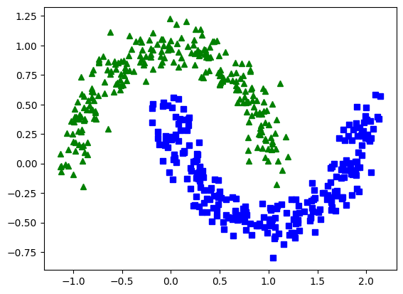
We test our implementation on the “moons” dataset—a classic 2D binary classification problem that creates two interleaving half-circles. This dataset is perfect for validating logistic regression because:

• Non-linear boundary: Tests the model’s limitations
• Clear visualization: Easy to interpret results
• Balanced classes: Fair evaluation metric
• Controlled noise: Adjustable difficulty

Dataset Characteristics

• Training set: 500 samples
• Test set: 1,000 samples
• Features: 2D coordinates (x, y)
• Noise level: 0.1 (moderate difficulty)

Experimental Setup

# Initialize model parameters
np.random.seed(0)
w = np.random.rand(X_train.shape[1])  # Random weight initialization
b = 0                                 # Zero bias initialization

# Training configuration
iterations = 200
learning_rate = 0.1

# Train the model
w, b, loss_history = train(w, b, X_train, y_train, iter=200, lr=0.1)

Results Analysis

Our implementation achieved impressive results on this challenging dataset:

Training Performance

• Final Loss: Converged to approximately 0.57-0.58
• Training Accuracy: 82%
• Convergence Pattern: Rapid initial descent with stable convergence

Loss Convergence Behavior

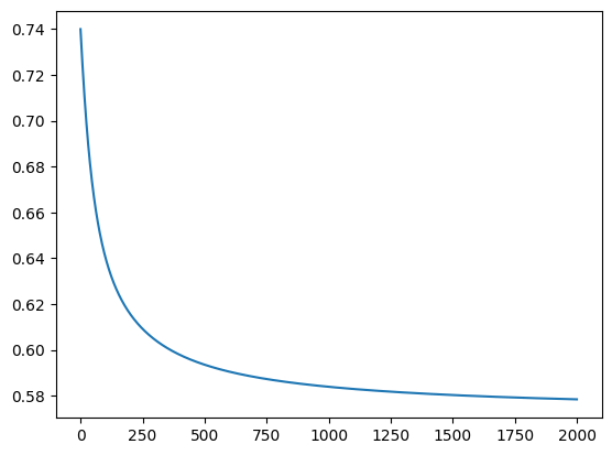
The loss curve reveals several interesting characteristics:

1. Rapid Initial Descent: Loss drops dramatically in the first 50 iterations
2. Non-Oscillatory Convergence: Even increasing the iterations to 2000, the loss remains positive
3. Stable Minimum: Reaches a stable plateau around iteration 200 iterations

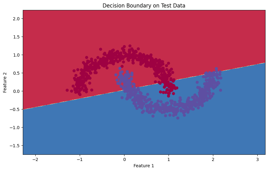
Model Limitations

A linear model will always be somewhat poor at predicting non-linear data. Specifically, the moons dataset requires a curved boundary to cleanly separate the two eponymous “moons”. As shown below, logistic regression cannot provide this.

Practical Applications

Understanding logistic regression is fundamental to more complex machine learning topics:

More Complex Models

• Neural networks: Logistic regression is essentially a single neuron (if using sigmoid as activation function)
• Deep learning: Multi-layer perceptrons build on these concepts
• Ensemble methods: Understanding base learners improves ensemble design

Real-World Scenarios

• Medical diagnosis: Binary classification (disease/no disease)
• Marketing: Customer conversion prediction
• Finance: Credit default risk assessment
• Text analysis: Spam detection, sentiment analysis

Whether you’re learning machine learning fundamentals or preparing to tackle more complex algorithms, this logistic regression implementation provides a solid foundation for understanding how optimization-based learning works under the hood.

The complete code and experimental setup are available here for further exploration and modification. Try experimenting with different learning rates, regularization techniques, or dataset variations to deepen your understanding!